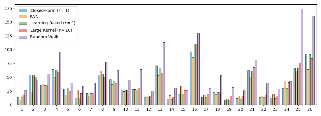
To evaluate the performance of our implementation we calculate the mean squared error on the unknown pixels of the benchmark images of [RRWGKR09].
Figure 1: Mean squared error of the estimated alpha matte to the ground truth alpha matte.
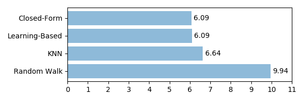
Figure 2: Mean squared error across all images from the benchmark dataset.
Visualization
The following videos show the iterates of the different methods.
Note that the videos of the slower methods have been accelerated.
CF
KNN
LKM
RW
Performance
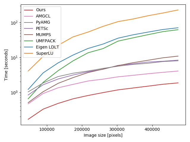
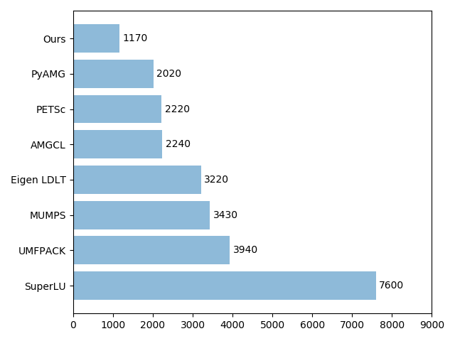
We compare the computational runtime of our solver with other solvers: pyAMG, UMFPAC, AMGCL, MUMPS, Eigen and SuperLU. Figure 3 shows that our implemented conjugate gradients method in combination with the incomplete Cholesky decomposition preconditioner outperforms the other methods by a large margin. For the iterative solver we used an absolute tolerance of \(10^{-7}\), which we scaled with the number of known pixels, i.e. pixels that are either marked as foreground or background in the trimap.
Figure 3: Comparison of runtime for different image sizes.
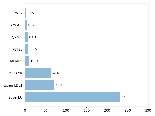
Figure 4: Mean running time of each solver in seconds.
Figure 5: Peak memory for each solver usage in MB.